Table of Contents
This tutorial is the example analysis with PoweREST on human intraductal papillary mucinous neoplasms (IPMN) data from GSE233254.
Required input data #
PoweREST requires 10X spatial transcriptomics data in Seurat format.
The example data for runing the tutorial can be downloaded here.
Load the package and data #
library(PoweREST)
three_areas <- readRDS("~/your_path_to_GSE233293_scMC.all.3areas.final")
Idents(three_areas)
# Levels: Peri Juxta Epi
The dataset has three histologically directed spot selection of epilesional, juxtalesional, and perilesional areas. We would like to perform the power estimation upon each of the three areas.
Preprocess data #
# Split the ST data by areas
SeuratObject_splitlist<-SplitObject(three_areas, split.by = "ident")

str(SeuratObject_splitlist[[1]][['Type']])
# Factor w/ 3 levels "LG","HG","IPMNPDAC"

# The original dataset has three cancer subtypes. According to the paper, 'HG' and 'IPMNPDAC' are combined into one 'HR' (high-risk) group
for (i in 1:length(SeuratObject_splitlist)) {
  SeuratObject_splitlist[[i]][['Condition']]<-ifelse(SeuratObject_splitlist[[i]][['Type']]=='LG','LG','HR')
}

# Set identity classes to the 'Condition' column in meta data
for (i in 1:length(SeuratObject_splitlist)) {
  Idents(SeuratObject_splitlist[[i]])<-"Condition"
}
Idents(SeuratObject_splitlist[[1]])
# Levels: HR LG
Power estimation though bootstrapping #
# First perform PoweREST upon 'Peri' area
Peri<-SeuratObject_splitlist[[1]]
Test Version: set ‘iteration’ to 5, ‘replicates’ is the sample size per group, ‘spots_num’ is the average number of spots across the tissue samples which in our case is 80.
test<-PoweREST(Peri,cond='Condition',replicates=5,spots_num=80,iteration=5)
Default Version: set ‘iteration’ to 100, it may take hours to run the code if iteration is 100 (default setting). We recommand you install presto by
install.packages('devtools')
devtools::install_github('immunogenomics/presto')
# then run this
result<-PoweREST(Peri,cond='Condition',replicates=5,spots_num=80,iteration=100)
Instead of using Wilcoxon test #
The default test in Seurat’s FindMarkers is Wilcoxon test. Users can specify any test avalible in FindMarkers function.
# For example, use the Student's t-test
result2<-PoweREST(Peri,cond='Condition',replicates=5,spots_num=80,iteration=100,test.use="t")
Power estimation upon a subset of genes #
Users can also use PoweREST_gene and PoweREST_subset to perform the power estimation upon one gene or a subset of genes. But be carefull when interpreting the results, since the power is based on the adjusted p-value after bonferroni correction.
PoweREST_gene performs the power calculation upon one gene by specifying the gene name.
one_gene<-PoweREST_gene(Peri,cond='Condition',replicates=5,spots_num=80,gene_name='MUC1',pvalue=0.00001)
PoweREST_subset performs the power calculation upon a subset of genes by specifying ‘logfc.threshold’ and ‘min.pct’ values.
sub_genes<-PoweREST_subset(Peri,cond='Condition',replicates=5,spots_num=80,pvalue=0.05,logfc.threshold = 0.1,min.pct = 0.01)
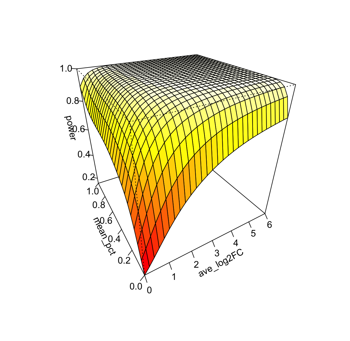
Fit power surface #
Here, we utilized penalized splines under two-dimentional constraints to fit the power surface.
# Fit the power surface for sample size=5 in each arm
b<-fit_powerest(result$power,result$avg_logFC,result$avg_PCT)

#Diagnosis the result
scam.check(b)

# Get the predition result
pred <- pred.powerest(b,xlim= c(0,6),ylim=c(0,1))
Visualize the surface #
vis.powerest(pred,theta=-30,phi=30,color='heat',ticktype = "detailed",xlim=c(0,6),nticks=5)
Create interactive visualization result #
plotly_powerest(pred,fig_title='Power estimation result')
Visualize two surfaces in one plot #
The following code uses the pre-calculated power estimation results of bootstraping resampled replicates ranging from 1 to 10.
power_values <- read.csv('./your_path_to_merge_long.csv')

# Power values of replicates=3
power1 <- dplyr::filter(power_values, sample_size==3)
b1 <- fit_powerest(power1$power,power1$avg_log2FC,power1$mean_PCT)
pred1 <- pred.powerest(b1,xlim= c(0,6),ylim=c(0,1))

# Power values of replicates=4
power2 <- dplyr::filter(power_values, sample_size==4)
b2 <- fit_powerest(power2$power,power2$avg_log2FC,power2$mean_PCT)
pred2 <- pred.powerest(b2,xlim= c(0,6),ylim=c(0,1))

fig <- plotly_powerest(pred1,fig_title='Power estimation result')
fig <- fig %>% add_surface(x = pre2$x, y = pred2$y,z = pred2$z,type = "surface",colorscale='BrBG',opacity = 0.3)
This code can be used to inspect any crossings between surfaces.
Fit local power surface with XGBoost #
XGBoost is used as a remedy when there are crossings between surfaces but is recommended to only fit the local power surface.
# Fit the local power surface of avg_log2FC_abs between 0 and 2
avg_log2FC_abs_0_2<-dplyr::filter(power_values, avg_log2FC_absolute<2)

# Fit the model
bst<-fit_XGBoost(avg_log2FC_abs_0_2$power,
                 avg_log2FC=avg_log2FC_abs_0_2$avg_log2FC_absolute,
                 avg_PCT=avg_log2FC_abs_0_2$mean_pct,
                 replicates= avg_log2FC_abs_0_2$sample_size)

# Make predictions
pred_xgb<-pred_XGBoost(bst,n.grid=30,xlim=c(0,2),ylim=c(0,1),replicates=3)
Visualize the local power surface #
#2D version
vis_XGBoost(pred_xgb,view='2D',legend_name='Power',xlab='avg_log2FC_abs',ylab='mean_pct')
#3D version
vis_XGBoost(pred_xgb,view='3D',legend_name='Power',xlab='avg_log2FC_abs',ylab='mean_pct')